Posts

Scale and Spatial Data Aggregation

Image
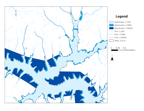
 Scale and Spatial Data Aggregation Levels of Detail In spatial data analysis, scale and data aggregation are critical factors that influence the outcome of geographic studies and decision-making processes. Both play a vital role in determining how geographic phenomena are recorded, represented, and understood.  Scale Scale in the context of spatial data refers to spatial extent or the level of detail that geographic features are recorded and represented. Scale can be understood as the ratio of what is featured on the map and what occurs in the real world. It is impossible to record every microscopic detail of the land or every nuance of nominal study features. Spatial analysts must determine the level of data smoothing required for a project.  In geographic studies, as scale changes, so too do the features of the landscape. The simple map below records water features for the same study area and compares them at three levels of scale. As coarseness increases, smaller features are lost

Spatial Interpolation

Image
Spatial Interpolation Comparing Exact Interpolators Interpolation is a fundamental concept in spatial analysis, where we aim to predict and construct new data within a range of known data points. In an ideal world, we could do field studies on every square centimeter of the Earth and collect unlimited data. Since this not (yet) possible, we can strategically plan where to collect samples and use these points to mathematically predict ground truth. But before that, here's a joke. Did you know there are two kinds of people in the world? (1) Those who can extrapolate from incomplete data What are Exact Interpolators? For this analysis, we compared several methods of exact interpolation techniques. Exact interpolators are methods where functions pass through known data points. We compared the outcomes of three differing methods: Thiessen polygons, Inverse Distance Weighting (IDW), and Spline (regularized and tension). While these methods guarantee accuracy at known points, choosing the

Surfaces - TINs and DEMs

Image
Surfaces - TINs and DEMs Triangulated Irregular Networks (TINs) and Digital Elevation Models (DEMs) provide models critical to understanding and analyzing our planet. Through ArcGIS Pro, the GIS platform developed by Esri, we can create both these model types. Understanding TINs and DEMs What is a TIN? A Triangulated Irregular Network (TIN)  is a vector-based surface representation, represented through the connection of elevation points. These irregular points are connected with non-overlapping triangles. The face of each triangle is interpolated for values such as slope.  TINs are effective models for representing rugged terrain while also being data light. Because values are derived from a finite number of points, the facet values are assumed. Subtle changes in the landscape are lost in exchange for efficiency. Close up of TIN model What is a DEM? A Digital Elevation Model (DEM)  is a raster-based representation of the earth's surface, where each raster cell (also called pixel) r

Data "Completeness"

Image
  Comparing Completeness In continuing our investigations of data quality, this week we look at data "completeness". How can we ensure that the information we are given is not just accurate but actually covers the areas we need? Going out to the field, making measurements, and taking the records ourselves would be time-consuming and exorbitantly expensive. Instead, we can compare our dataset with a higher-quality dataset.  For this project, we were tasked with comparing the completeness of Jackson County, Oregon's road network to the federally recognized network. The US Census Bureau's TIGER (Topologically Integrated Geographic Encoding and Referencing) linefiles are a reliable dataset, which we will use as the control variable in this analysis. The method for this analysis is in reference to Haklay's 2010 study, " How good is volunteered geographical information? A comparative study of OpenStreetMap and Ordnance survey datasets".           County road n

Spatial Data Standards

Image
Testing For Spatial Data Standards This week's lab continued exploring data quality by completing an analysis of horizontal accuracy for two different datasets from 2006. Two different shapefiles were delivered to us: one from the city of Albuquerque itself and the other from TeleAtlas' StreetMap USA. We were also given 6x6 orthophotos of the study area. Initially, twenty reference sites were chosen using ArcGIS's geoprocessing tool Create Random Points with a minimum distance of 5,000 feet between each site. These reference points were then manually adjusted to the nearest "ideal" street intersection as seen on the orthophotos. Ideal locations contained clear, simple intersections with 90-degree intersections. Street intersections provide precise and unambiguous locations that can be easily identified. They are also consistent over time and can be repeatedly located with high precision. Next, test points were created for each dataset along the provided polylines.

Precision and Accuracy

Image
  Three statisticians go duck hunting. The first statistician shoots and misses just left of the duck. The second statistician takes aim, shoots, and misses just right of the duck. The third statistician jumps up in joy and shouts, "We got 'em!" Before any spatial project can be underway, a thorough analysis of measurement quality is essential. Accuracy refers to the truthfulness of a measured value. Relatedly, precision refers to the consistency of measurements. Repeated measurements of similar value indicate minimal random error.  A reliable analysis requires both accuracy and precision. It is critical then to check for variability and potential bias. In this scenario, data validity was performed on horizontal accuracy and precision.  Fifty (50) survey points were provided to us. First, we checked for precision by calculating the average of the repeated measurements. A new average point feature class was created by calculating the mean longitude and latitude of all 50 p

Pregnancy and Birth in the United States: Comparing Infant and Maternal Mortality Rates Across 29 OECD Countries, 2019-2021

Image