Hot Spot Crime Analysis
Hot Spot Analysis: Using Spatial Analysis Tools to Identify, Target, and Predict Criminal Activity
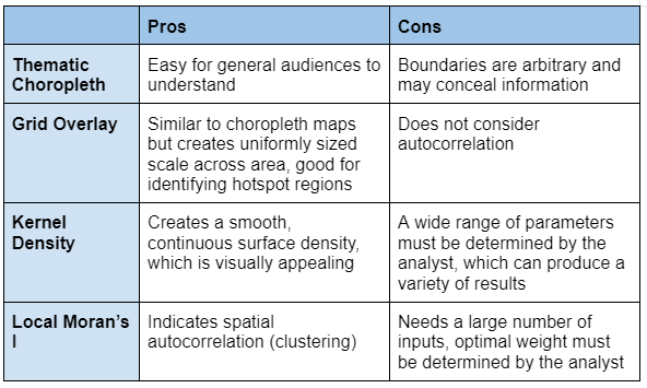
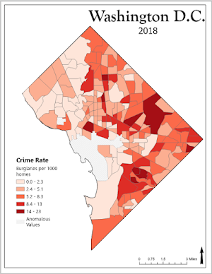
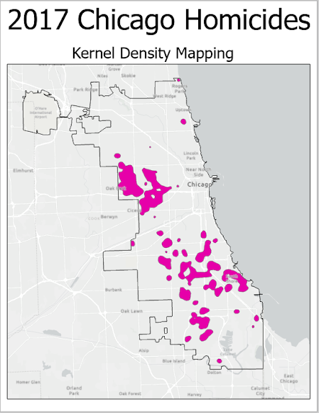
Hotspot analysis is a spatial analysis tool that identifies areas of unusual density. There are many methods for identifying these clusters but the most common are thematic choropleth maps, kernel density, and Moran's I. Hotspot analysis is of particular interest to the criminal justice field as police departments and political leaders are interested in targeting areas with high crime rates. As demonstrated in the two maps below, how crime hotspots are represented can dramatically alter interpretation and future policy decisions.
Major Types of Hot Spot Analysis:
Grid Overlay Mapping
First, the grid cells feature class was joined with the total number of homicides (2017), which provided us a joint count of homicides per cell. I exported only the cells containing one or more homicides to a new feature class called “homicide_count” with the expression [join_count > 0]. After sorting from highest to lowest, the top 20% of grid cells were selected (rounded down to 62 total) and exported to a new feature class called “hom_top20per”. A new field was added and calculated for the integer one. Dissolve was performed on all remaining cells to create one new, single feature.
Kernel Density
Through the geoprocessing tools in ArcGIS Pro, a kernel density analysis was performed on the 2017 homicides class. The output cell size was set at 100 feet with a search radius of 2,630 feet (1 US mile). The symbology of the new raster layer was then adjusted to Natural Breaks (Jenks) with two classes. The classes were manually set at 3*mean (3*2.88=8.64) and more than 3*mean (>8.64 to 38.92). By using the reclassify tool, the raster was given two values (1 and 2). The file was then converted to a polygon layer. All grids labeled as two were exported to a new class (hom_kd), which was used as our final hotspot result.
Local Moran's I
Similar to grid overlay mapping, a spatial join of the census tracts and the 2017 homicide table was performed to produce homicide counts per tract. A new field was added to calculate the crime rate per 1,000 households (Crime_Rate = join_count / total households * 1000). The cluster and outlier analysis tool was used to create a new output feature class, which classified areas of high-high, high-low, low-high, and low-low crime. The high-high clusters were exported to their own feature class, which was then dissolved into a multipart feature.



Comments
Post a Comment