Assessing Suitability

Suitability Analysis: Booleans in Vectors & Rasters

An important product of GIS is identifying areas that fit a range of criteria. Where should the local city focus its limited resources? Where can ecologists find a rare species? How do we make the best choice when time and money are on the line? 

In GIS, we can attempt to answer these questions with a suitability analysis, which provides a framework for picking "the best" locations for our needs. 

Suitability analysis (also called a multicriteria decision analysis) consists of criteria and objectives, the corresponding layers, and a composite of all layers. In other words, there is a problem that needs to be solved, information related to that problem, and a system of making a final result that considers all of the required objectives.

So what does that mean in the real world? For the following example, we were asked by wildlife experts to help create a map where mountain lions (cougars) could be located. For this objective, we need to know the ideal environment for mountain lions. We are told they like steep slopes; sources of flowing water nearby; forest coverage; and a distance between them and human development. If the location checks all of these requirements, we might find ourselves a big kitty.

Public Domain

We have been provided layers of information for each criterion:

• Objective 1: Locate where there are steep slopes (more than 9 degrees)
• Objective 2: Locate areas covered by forest (code 41, 42, 43)
• Objective 3: Locate areas more than 2,500 feet away from highways
• Objective 4: Locate areas less than 2,500 feet from a river
• Objective 5: Constrain results to the provided study area

Creating a flowchart will help us stay organized as we're about to produce a lot of data. Each layer will need to be manipulated to find only the suitable locations. 

Slope

The DEM is measured for slope in degrees with the Slope tool. The resulting measurements are then reclassed into less than 9 degrees and more than 9 degrees. We will want just the steep slopes later in our analysis, so these are assigned a value of 1. Areas we do not want are given a value of 0.

All slope measurements (left) are sorted into our yes/no categories (right).

Land Cover

We repeat the reclassing process for land cover to select for forested areas. All forested areas are given a value of 1 whereas all the non-forested land is given a value of 0. Sorting by 0/1 is a mathematical expression of yes/no.

All landcover types are sorted into a binary layer,

Rivers and Roads

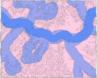
The buffer tool generates polygons of locations within 2,500 feet of either a road or river. Areas near rivers are reclassified as 1 (yes) and areas near roads are assigned 0 (no). Areas too far from rivers are given the value 0 (no) and areas sufficiently away from roads are assigned 1 (yes).

Buffers (zones) are created around rivers and roads.

Final Selection

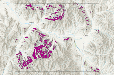
Now we can make a final selection by using SQL, where the final output contains only the 1 (yes) values. Below are the areas that meet all of our requirements.

We could also perform a Union (for rasters) or Combine (for vectors) on the boolean layers to create a map that shows more details. Each shaded area below represents a number of achieved criteria. Perhaps the researchers had no luck finding mountain lions in the ideal zones. The map below shows us where the next ideal search areas are located.

Weighted Suitability

The above scenario assumes only a yes/no (also called boolean) checklist. However, we know the real world is rarely in black and white. We can adjust our criteria to reflect levels of importance by "weighting" them. These are also called ranked or scored choices.

In the next scenario, a property developer is interested in, well, developing some property. They want to find the ideal places to build based on land cover, soil type, slope, stream distance, and road distance. The most suitable locations will be clear of trees, wetlands, and urban development; a soil type with drainage but not prone to erosion; little to no slope; and away from streams but close to road access. 

For each layer, we assign attributes with a ranking of 1-5, with 1 being the least suitable and 5 being the best. Each layer is then combined using the Weighted Overlay tool. In Scenario 1, we specify each layer as having the same weight (20%). In Scenario 2, we assigned a variety of weights:

• Land cover -- 20%
• Soils -- 20%
• Slope -- 40%
• Distance to streams -- 10%
• Distance to roads -- 10%